Crashworthiness Analysis of an Automotive Front Rail in Abaqus

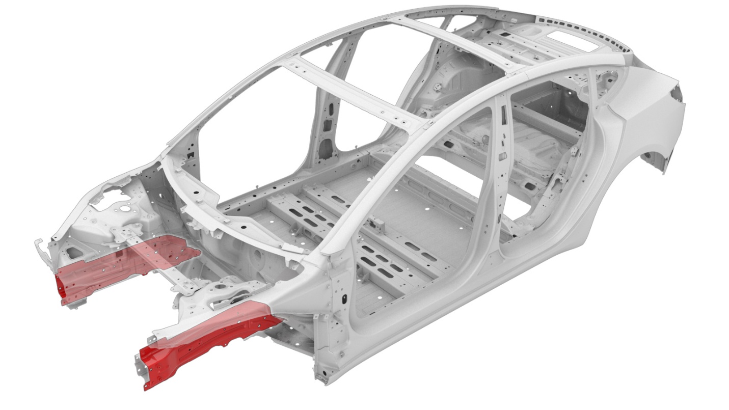
This is my lab record for the Computational Solid Mechanics course in the Spring 2026 semester.

The Importance of Automotive Front Longitudinal Rails

In a frontal collision of a passenger car, the front longitudinal rail first bends, buckles, and progressively folds layer by layer. As the metal deforms permanently beyond its original shape, a portion of the vehicle’s kinetic energy is converted into plastic deformation. Our Computational Solid Mechanics course project required us to investigate the front longitudinal rail, treating it as the primary component responsible for absorbing roughly half of the vehicle’s kinetic energy in a frontal crash. The assignment given by the instructor was open-ended and provided several exploratory directions:

• Simulate the dynamic impact of the front longitudinal rail;
• Reference curved beam examples to learn modeling and post-processing methods;
• Start from the provided STEP geometry;
• Plot force–displacement curves;
• Finally, explore different cross-sectional shapes.

The instructor did not strictly specify parameters such as material, impact velocity, impactor mass, mesh size, or how many configurations to evaluate—these decisions were left up to us. Our goal was straightforward: how can we achieve progressive folding in the rail to absorb more kinetic energy without generating excessively high peak forces during initial contact?

Standardizing Model Units and Scale

The provided baseline rail geometry is 1000 mm long. The baseline top-hat cross-section has a total width of 100 mm, an inner span of 59 mm, a total height of 51.2 mm, and flange widths of 20.5 mm. The top-hat section has a thickness of 1.2 mm, and the closing plate has a thickness of 0.8 mm. Subsequent variations—such as setting both parts to a uniform 1.0 mm thickness or thickening the corners—were all derived from this baseline.

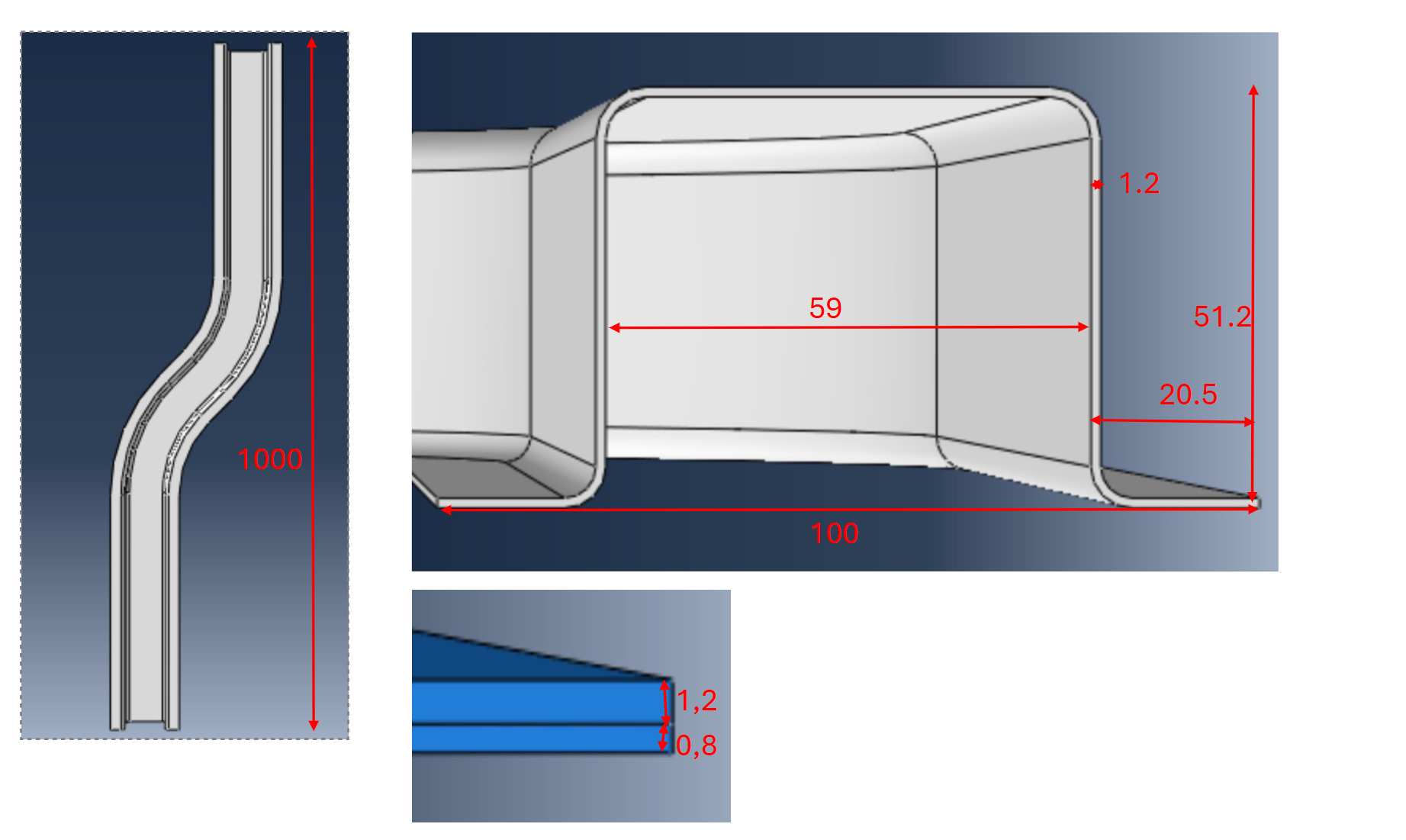
The simulation uses the consistent mm–tonne–s unit system: length in mm, force in N, mass in tonne, time in s, and stress in MPa. This unit system is easiest to misinterpret when reading energy outputs: Abaqus outputs energy in N·mm, not in Joules (J).

Quantity	Unit
Length	mm
Force	N
Mass	tonne
Time	s
Stress	MPa (N/mm²)
Energy	N·mm

$$1\times10^6\ \text{N·mm}=1\ \text{kJ}.$$

The area under the force–displacement curve represents the work done:

$$W=\int F\,dx.$$

Therefore, $3.5\times10^6$ N·mm on the plot is actually 3.5 kJ and cannot be written as $3.5\times10^6$ J.

Once the dimensions and units were aligned, we ran our first round of simulations and immediately encountered missing property assignments.

Round 1: Initial Setup

Identifying the Issue: 328 Elements Missing Section Properties

When inspecting the initial model file, we discovered that 328 elements had no material or section properties assigned. Abaqus halted during the input check stage, producing no crash results. While this error was fundamental, it was a valuable lesson: having parts, meshes, and jobs defined in the model tree does not mean the solver is actually computing. From then on, we checked every section assignment before submitting any job.

Early Baseline

The early baseline impact velocity was 13,888 mm/s (approximately 50 km/h).

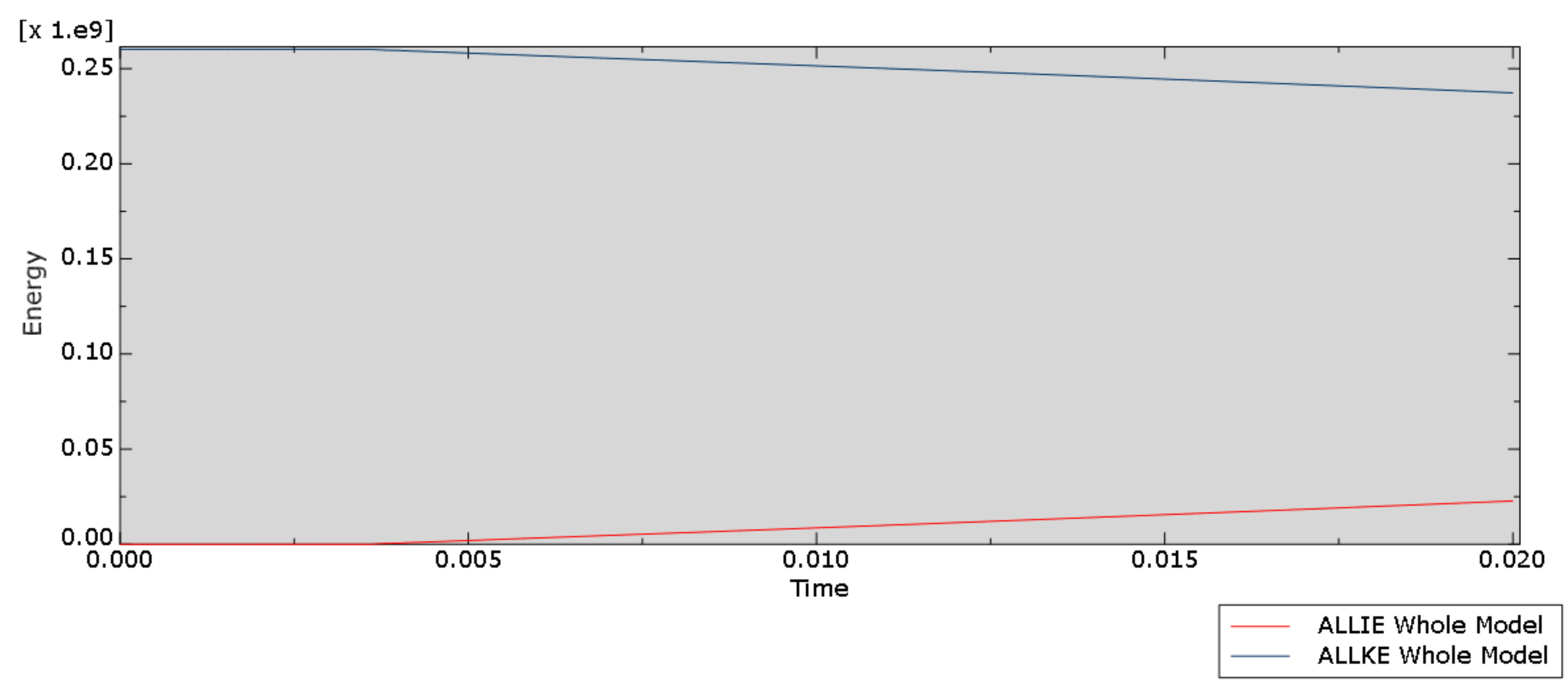
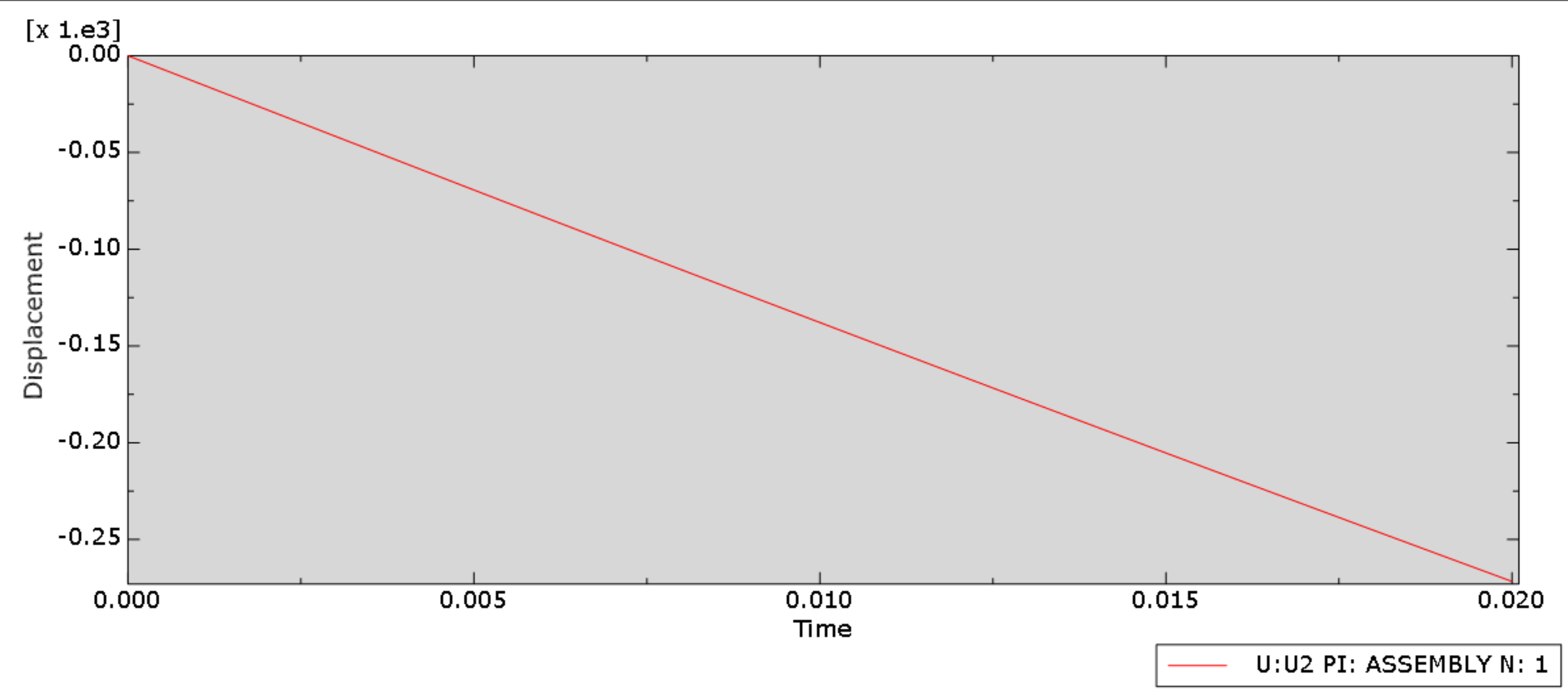
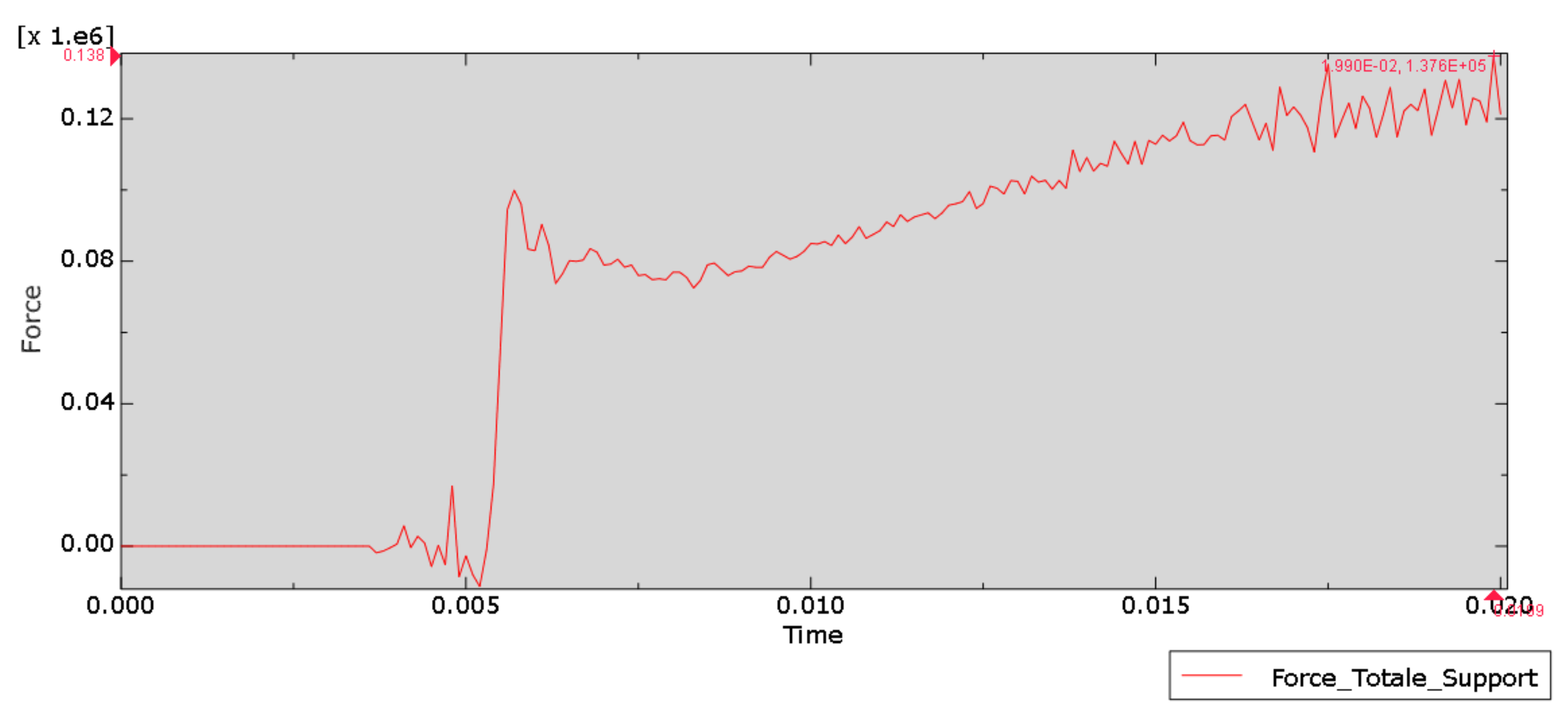
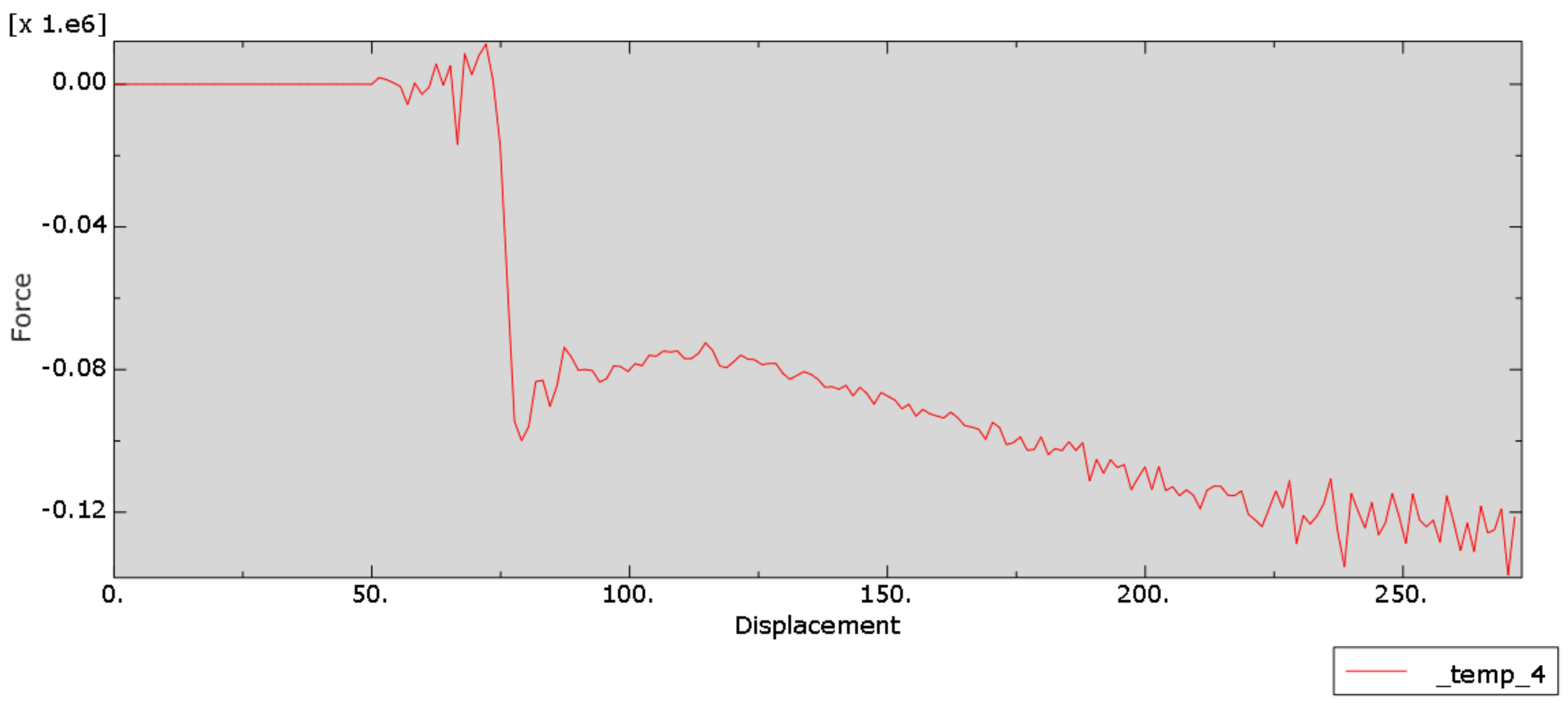
During the first 0.005 s, the impactor has not yet made contact with the rail, so the reaction force remains near zero. Upon contact, an initial peak force of approximately 100 kN appears, followed by continuous folding of the rail as the reaction force oscillates and rises, reaching 137.6 kN around 0.0199 s. The impactor traveled about 270 mm in 0.02 s along a nearly linear trajectory, indicating that its velocity had not yet dropped significantly during this interval.

The raw force curve exhibits substantial high-frequency oscillations. Explicit integration, contact algorithms, stress waves, and mass scaling all introduce numerical oscillations into the output. We retained the raw curves to monitor instantaneous peak values, while using filtered curves to evaluate the overall force plateau, rather than selecting only the cleaner-looking plot.

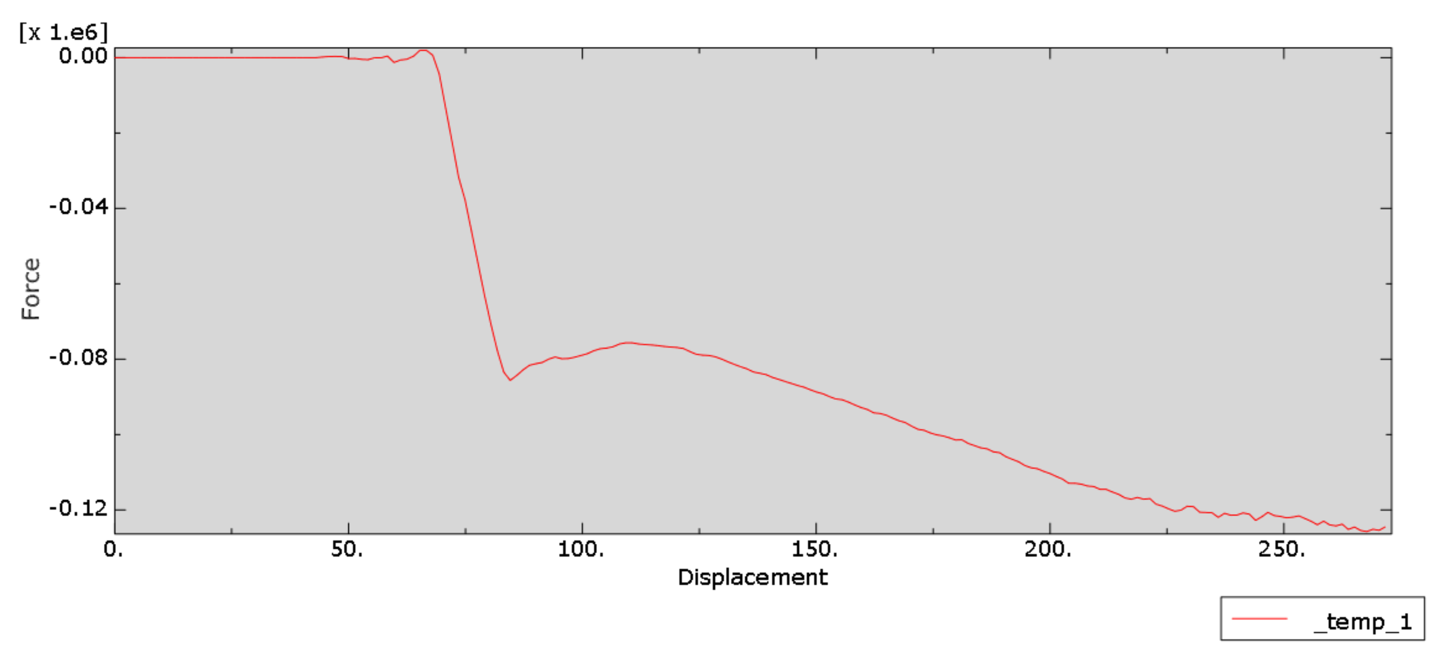
After assigning the missing section properties, we moved on to explore V2.

Round 2: Exploring Materials

The V2 model was updated to 393 C3D8R elements and 902 nodes, maintaining the velocity of 13,888 mm/s with an extended analysis duration of 0.04 s and a contact friction coefficient of 0.3. A total of four jobs were completed.

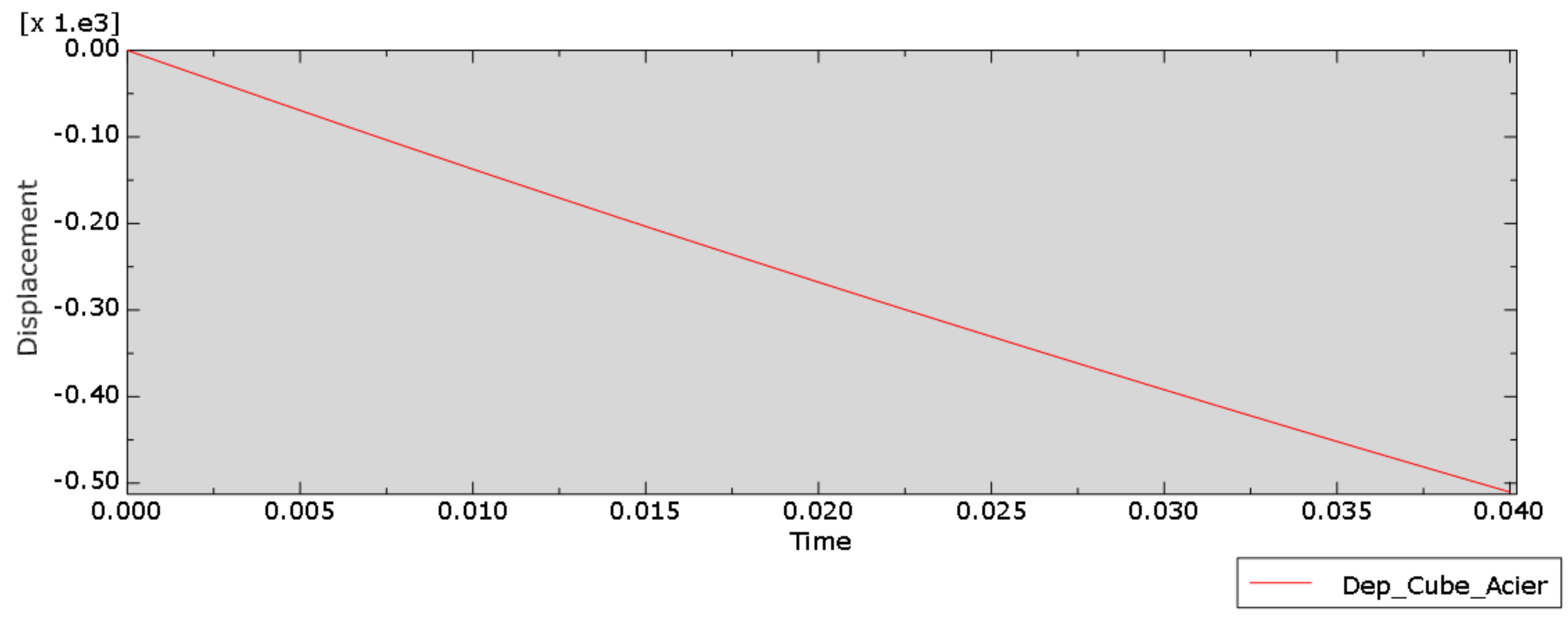
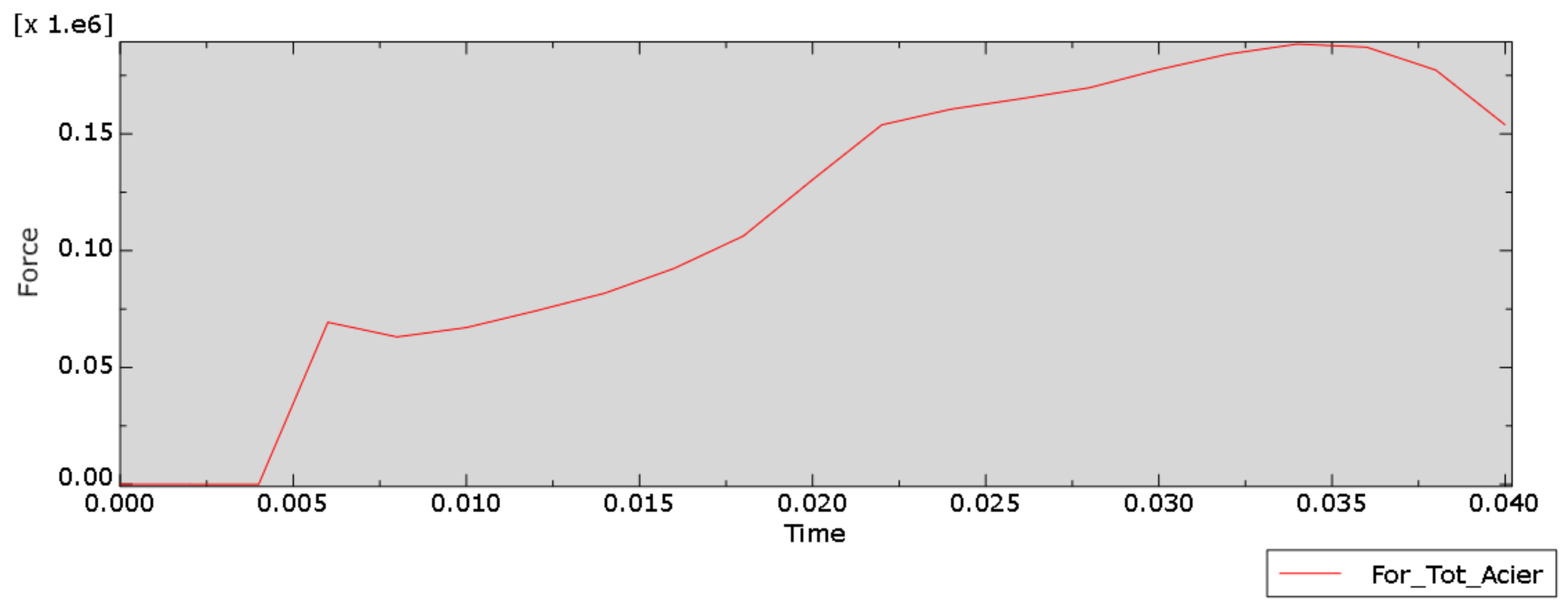
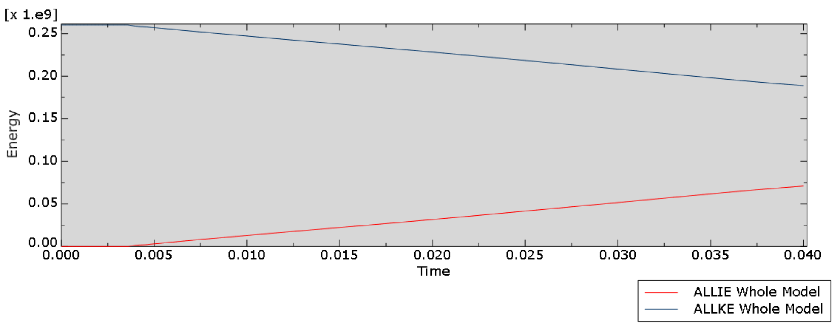
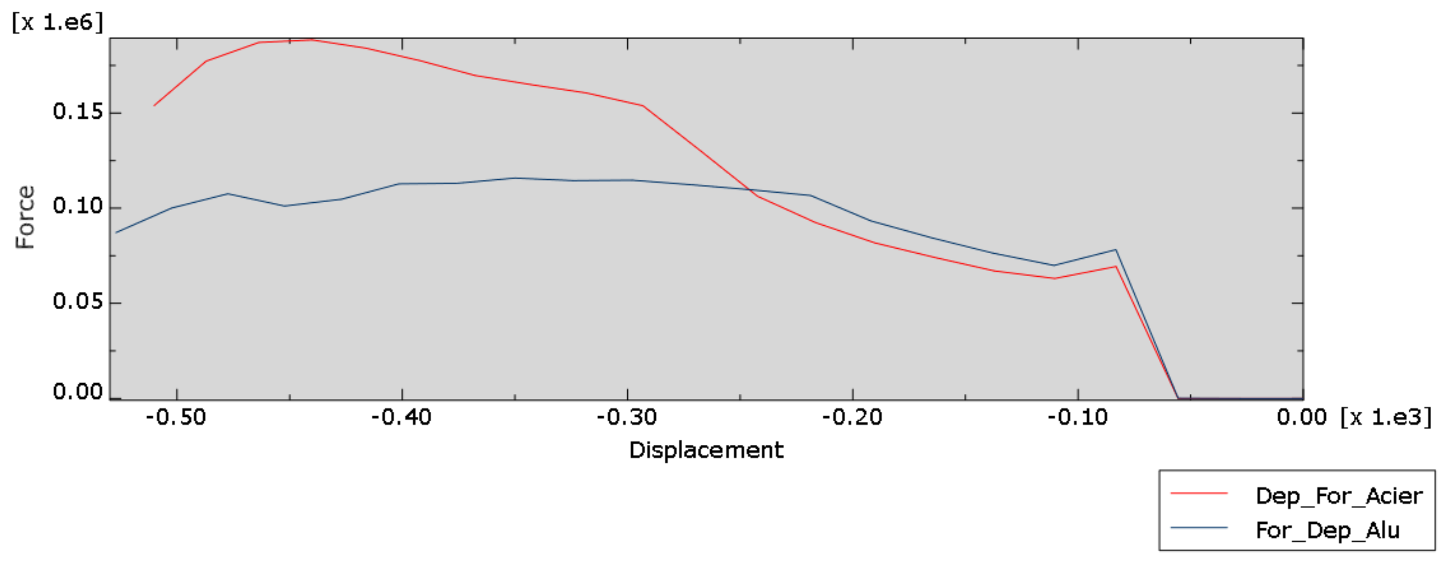
Looking first at steel: the impactor displaced approximately 500 mm in 0.04 s, with the reaction force rising to roughly 190 kN; as kinetic energy decreased, internal energy increased correspondingly.

Aluminum exhibited a lower peak force, around 115 kN. The stress contours show high concentrations in the bending and folding zones, which is precisely where thin-walled structures absorb energy via localized plastic buckling.

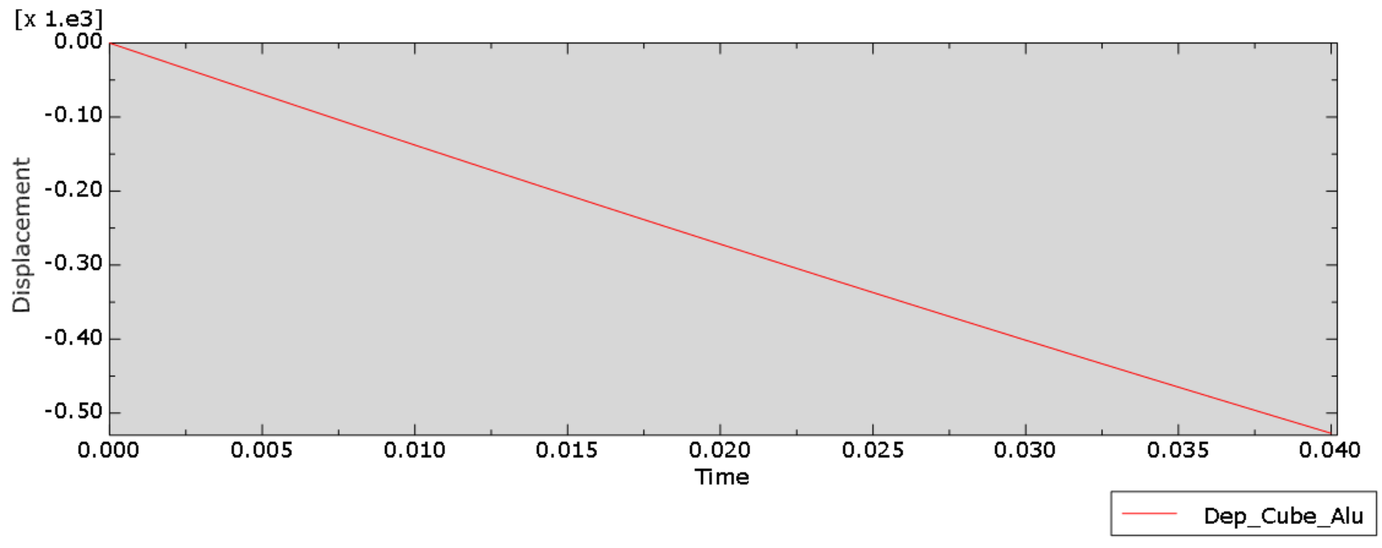
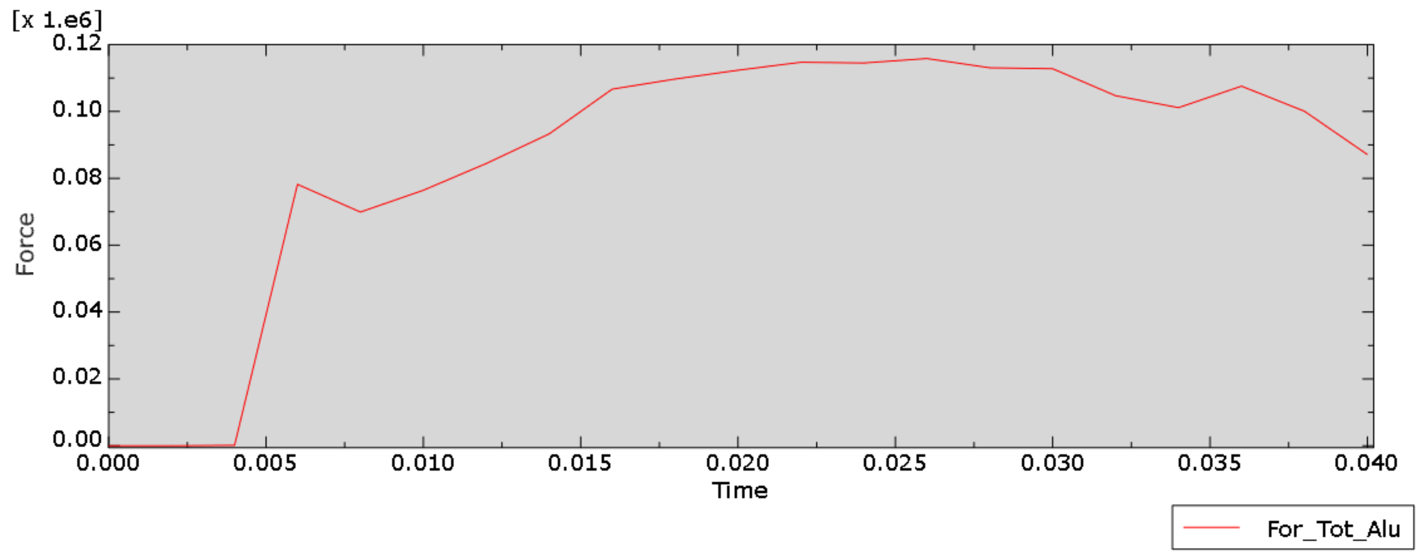
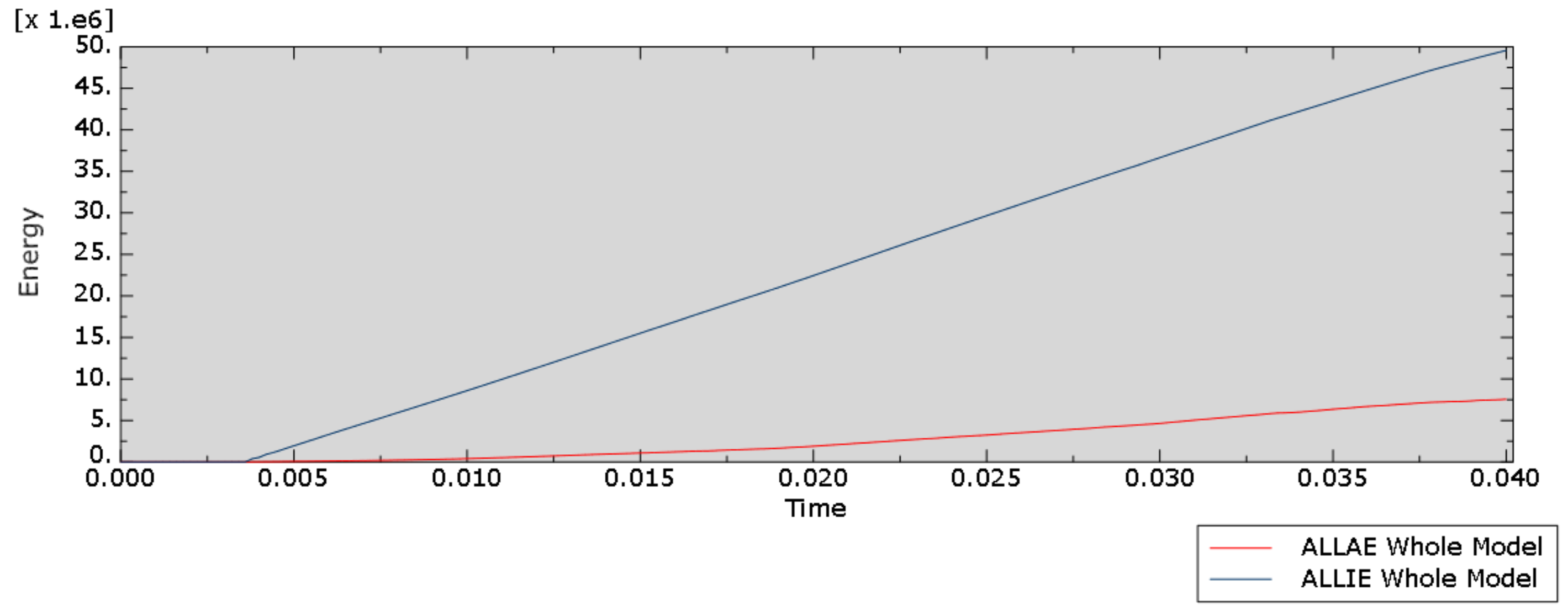
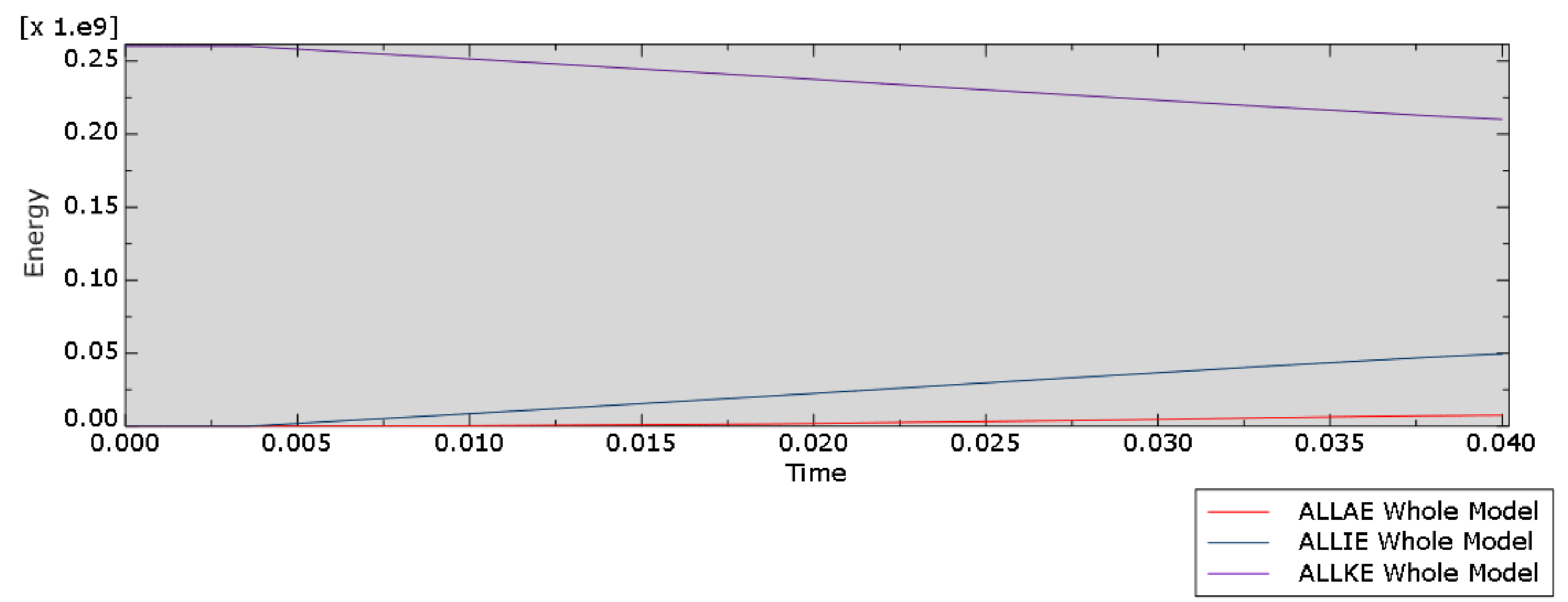
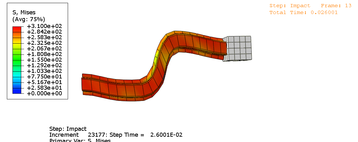
Comparing steel and aluminum on the same force–displacement plot, steel peaked at roughly 190 kN, while aluminum peaked at around 115 kN. Integrating the curves yielded total work values of approximately 58 kJ and 46 kJ, respectively. The density of steel is 7850 kg/m³, compared to 2500 kg/m³ for aluminum. Assuming identical geometric volume and converting by mass, aluminum achieved a Specific Energy Absorption (SEA) roughly 2.48 times higher than steel. Steel absorbed more absolute energy, while aluminum delivered a substantial portion of the work at a significantly lower mass.

Some energy plot values did not perfectly align with the integrated force–displacement work. In V2, we had applied a fixed mass scaling factor of 100, which increased mass by approximately 9900%; by the end of the aluminum simulation, $ALLAE/ALLIE\approx15\%$, indicating non-trivial artificial energy. Magnesium exhibited a reaction force plateau around 70 kN, which served as an initial data point. To make rigorous material comparisons, geometry, mesh, velocity, and impactor mass must be held constant, and excessive mass scaling must be removed.

While these results provided clear directional insights, their numerical quality needed improvement. We decided to switch to a 500 kg rigid impactor setup to verify whether the material trends persisted under more controlled conditions.

Re-evaluating with a 500 kg Impactor

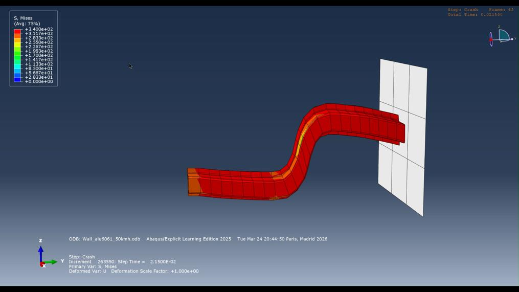
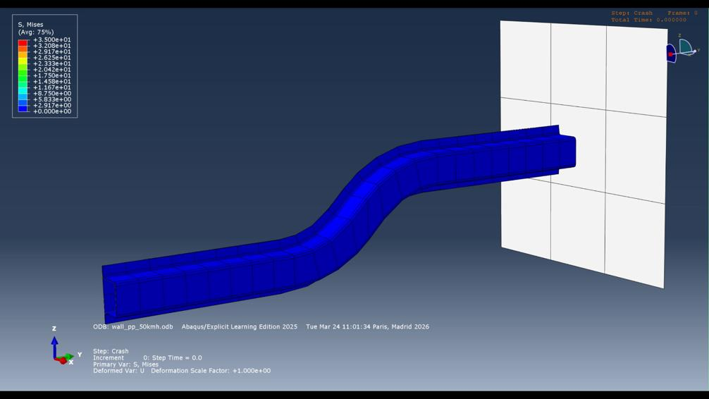
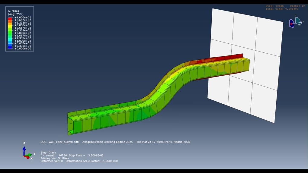
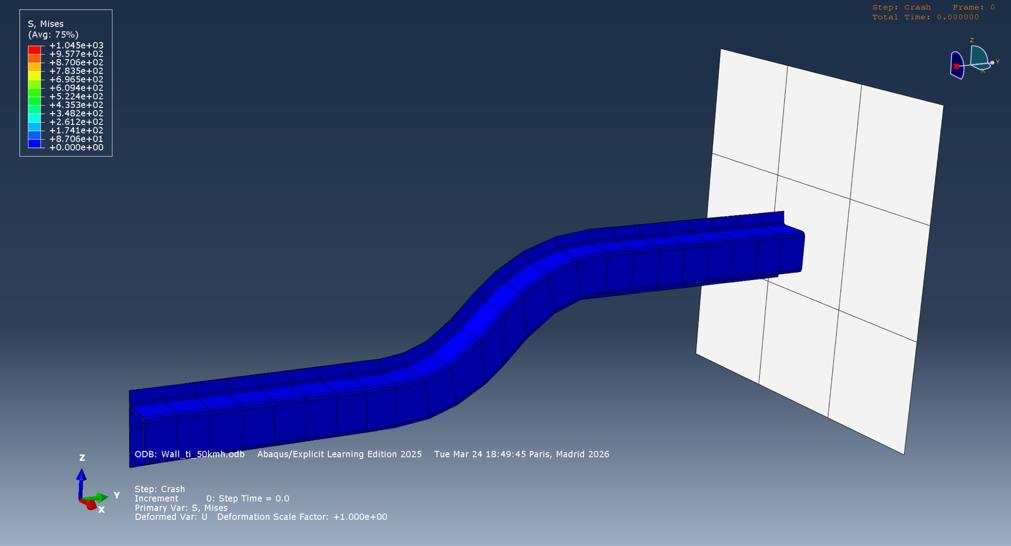
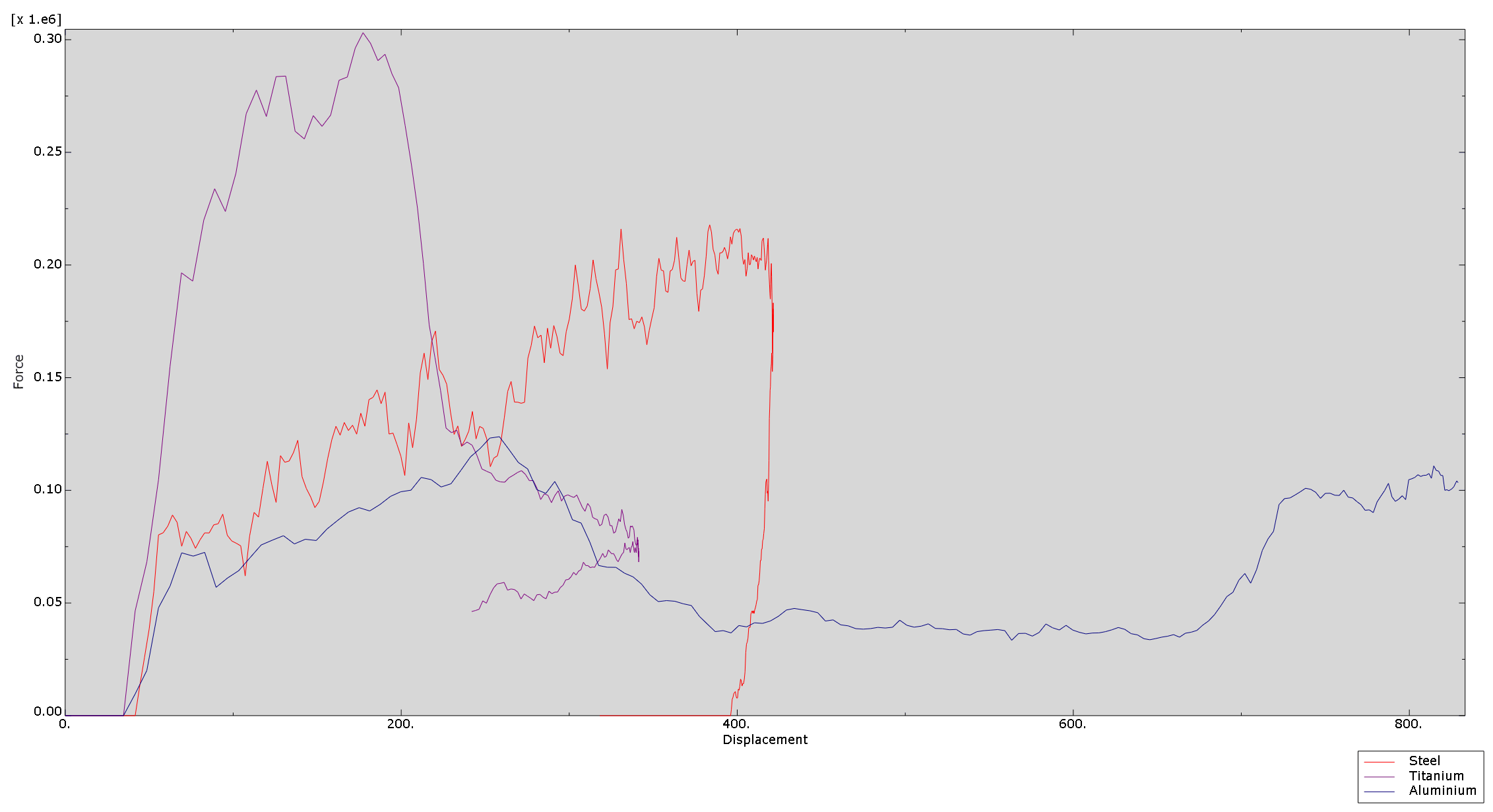
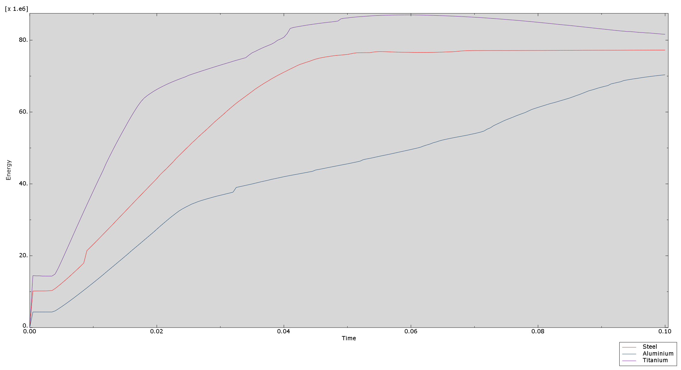
We set up a separate rigid wall impact study using a 500 kg rigid impactor at 50 km/h against the absorber, testing steel, Al 6061, Ti-6Al-4V, and polypropylene. This model group used different mass, boundary conditions, and stroke constraints compared to V2, V3, and the A/B/D cross-section studies.

Material	Mass (kg)	Peak Force (kN)	CFE	SEA (kJ/kg)	Stroke (mm)
Steel	2.73	185	95.2%	17.3	268
Al 6061	0.94	102	60.5%	50.8	774
Ti-6Al-4V	1.54	249	92.5%	27.9	186

Polypropylene suffered from contact instability, making its force history unreliable, so it was excluded from the table. Al 6061 showed the lowest peak force and the highest SEA, but required a 774 mm deformation stroke—nearly triple that of steel. If the vehicle front structure cannot accommodate such a long crush stroke, a high SEA alone cannot resolve packaging constraints. Titanium alloy and steel demonstrated flatter plateaus, but at the cost of higher forces. Therefore, design evaluation cannot rely solely on the highest single metric in a table.

Both material test rounds showed that evaluating designs purely on peak force or SEA can easily lead to misleading conclusions. We paused material rankings and set up a clean 30 km/h baseline configuration.

Round 3: Completing the 30 km/h Impact Baseline

Model V3 returned to a 30 km/h impact condition. The top-hat rail and closing plate were both set to 1.0 mm thickness and joined using a Tie constraint; contact was modeled via General Contact with a friction coefficient of 0.3. The model consisted of 405 deformable elements, 961 nodes, a 1.0 tonne (1000 kg) rigid wall, an initial velocity of 8333 mm/s, and a simulation duration of 0.06 s. V3 ran to completion without fixed mass scaling.

Results showed an initial total energy of approximately 34.72 kJ and a final total energy of roughly 34.70 kJ, showing negligible energy drift. Residual kinetic energy was 22.65 kJ, indicating that about 12.07 kJ of kinetic energy was converted into other energy components. However, this 12.07 kJ cannot simply be assumed to be entirely plastic dissipation. To understand where the energy went, internal energy, artificial energy, contact energy, and other components must be examined item by item in the ODB.

V3 also left behind numerical considerations: the simulation exceeded 300,000 increments, and Abaqus recommended re-running with double precision. While it avoided the aggressive mass scaling of V2, we had not yet performed a mesh convergence study, so total energy conservation alone does not guarantee full numerical precision for every variable. With V3 running reliably, our focus shifted from “can the model solve” to “where should the limited material be placed?”.

Round 4: Exploring Cross-Section Modifications

Uniformly thickening a cross-section is the simplest approach, but not all regions of a thin-walled member contribute equally to crash performance. Folding typically initiates at corners and rib intersections, where plastic hinges form. The core concept of Functionally Graded Thickness (FGT) is to place more material at these critical regions while thinning flat, less-stressed walls, guiding localized buckling to develop in an orderly sequence.

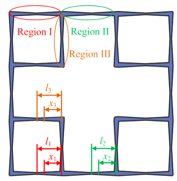
We referenced the study by Fang et al. (2015) in the International Journal of Mechanical Sciences, titled Dynamic crashing behavior of new extrudable multi-cell tubes with a functionally graded thickness. The paper divides the cross-section into three regions: Region I comprises the outer walls of corner elements, Region II consists of outer walls connecting corners, and Region III represents internal ribs. Theoretically, thickness transitions continuously from $t_{max}$ at the corners to $t_{min}$ along flat walls:

$$t(s)=t_{min}+\left(t_{max}-t_{min}\right)\left(1-\frac{s}{H}\right)^{n_i}.$$

Here, $s$ is the distance along the section wall, $H$ is the length of that wall segment, and $n_i$ governs the thickness gradient rate. The objective of this formulation is not to uniformly thicken the entire rail, but to redistribute material to where it is needed most under a constant mass constraint.

The paper implements a continuous thickness FGT design. In Abaqus, we implemented a simplified discrete approximation: 2 mm at the corners and 1 mm along the walls. We did not formulate a continuous thickness function nor perform a parametric optimization under strict constant mass. Model D is therefore an FGT-inspired multi-cell cross-section with stepwise thickness grading.

The animation below shows the original FGT deformation from our presentation. As deformation progresses at the central fold, the Mises stress contours shift progressively from blue to green, orange, and red.

Comparing Model A, B, and D

We evaluated three cross-sectional configurations:

• Model A (Classic): The original structure provided in the course, consisting of a top-hat channel and a flat closing plate joined into a single-cell section (top-hat 1.2 mm, closing plate 0.8 mm).
• Model B (Uniform): Retains the single-cell top-hat geometry of Model A, but sets both the top-hat and closing plate to a uniform 1.0 mm thickness to evaluate whether uniform wall thickness improves crush stability.
• Model D (FGT-Inspired Multi-Cell Section): Replaces the single cell with internal ribs and partitions forming a multi-cell cross-section. Corners are 2 mm thick and flat walls are 1 mm thick, concentrating material at plastic hinge locations.

All geometric comparisons were evaluated at $t = 0.06$ s. A uniform 2 mm Model C was also tested, but lacked complete final output data and was excluded from the summary table.

Metric	Model A	Model B	Model D
Mass (kg)	0.727	0.683	3.397
ALLIE (kJ)	3.5	2.8	33.0
Residual Kinetic Energy (kJ)	31.0	32.0	0.5
ALLAE/ALLIE	<1%	<1%	<1%
SEA (kJ/kg)	4.81	4.09	9.71
Peak Force (kN)	32.0	32.5	280
Mean Force (kN)	11.6	7.7	264
CFE	36.2%	23.7%	94.3%
Max Displacement (mm)	300	360	125

Model A: Baseline Allows Substantial Residual Travel

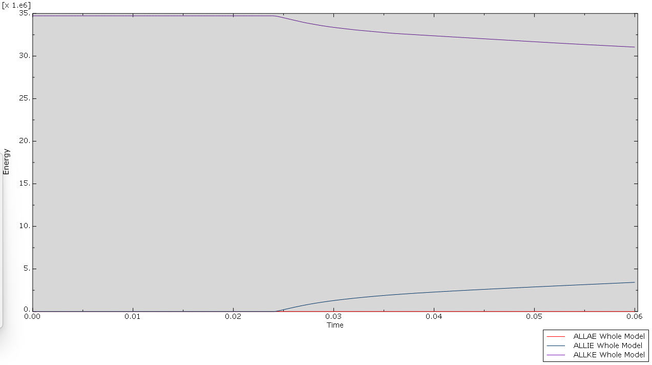
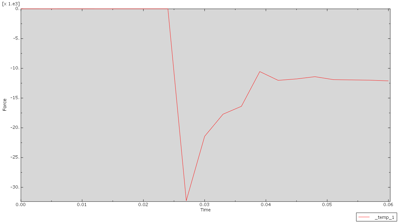
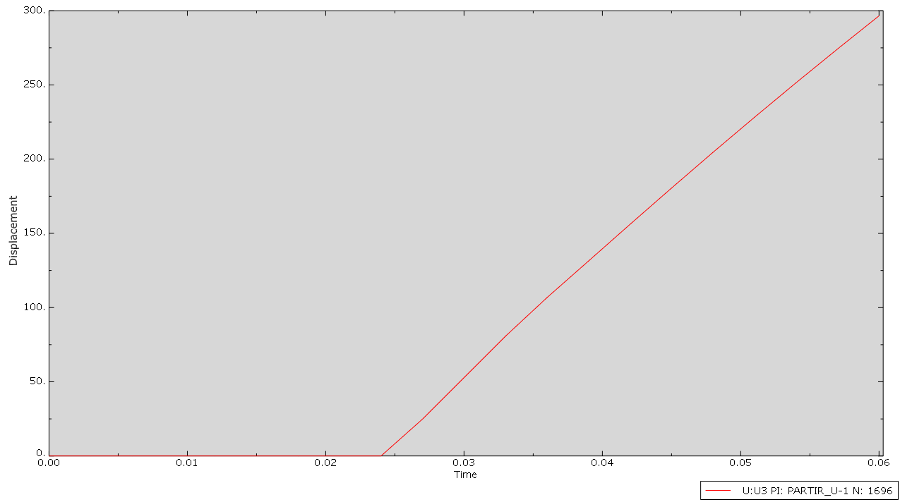
Model A reached an internal energy of 3.5 kJ, a mean force of 11.6 kN, and a peak force of 32 kN, with 31 kJ of residual kinetic energy remaining after 300 mm of travel. It established an easily understood baseline.

Model B: Uniform 1.0 mm Thickness

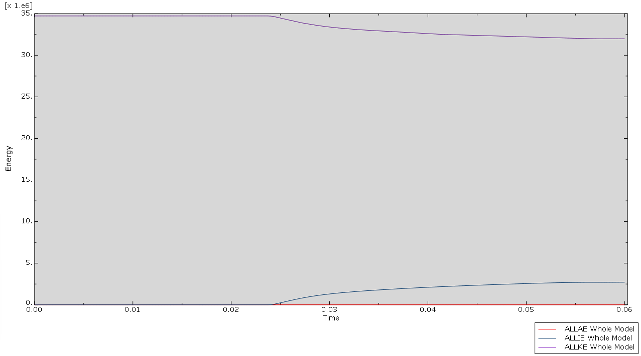
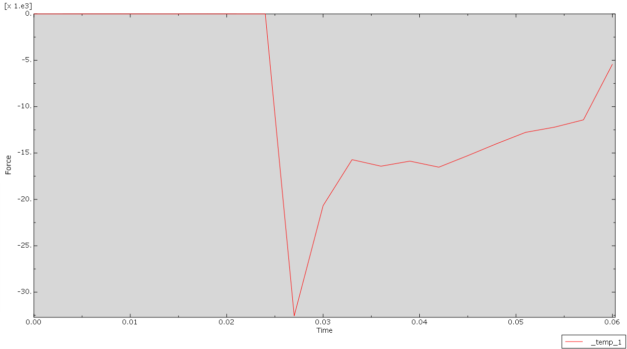
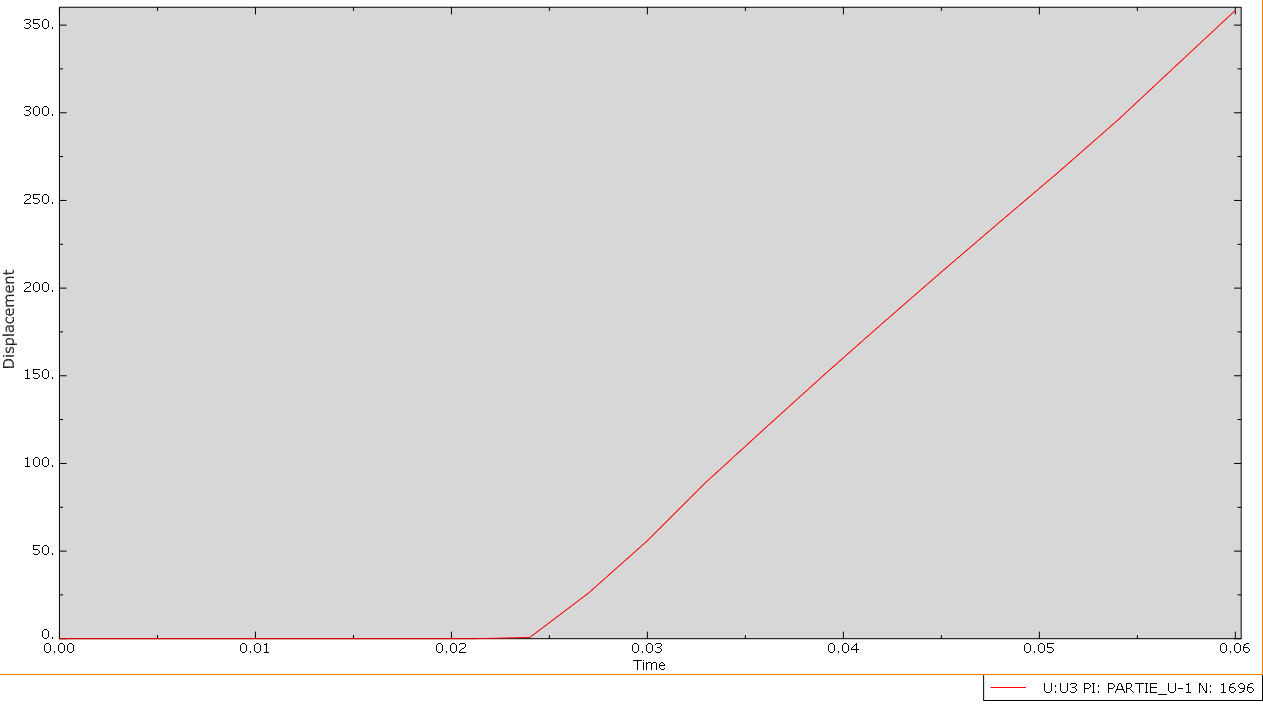
Switching from Model A to Model B reduced mass by only 6.1%, but ALLIE decreased by 20%, SEA dropped by 15%, mean force decreased by 33.6%, CFE dropped by 12.5 percentage points, and displacement increased by 20%. This does not imply that 1.0 mm thickness is inherently worse; rather, redistributing thickness altered the initiation and sequence of folding.

Model D: Multi-Cell Section with Thickened Corners

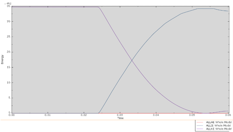
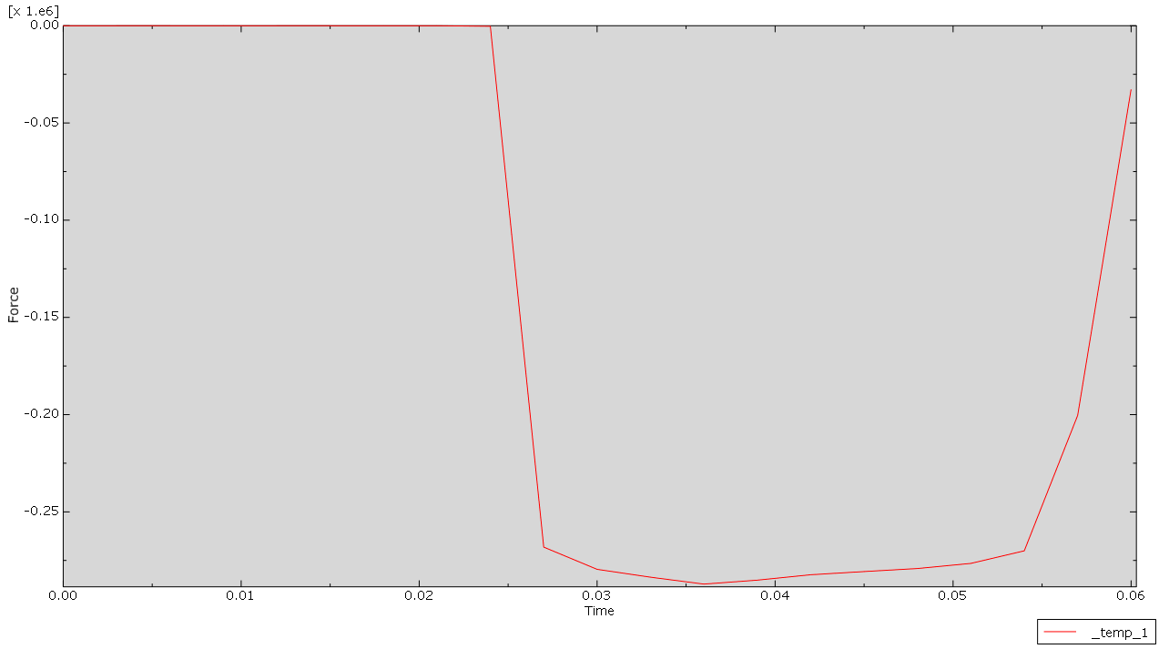
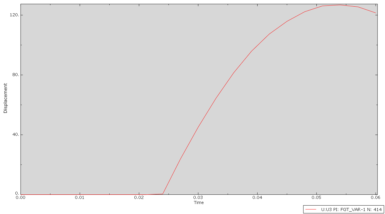
Transitioning from Model A to Model D increased mass by 4.67×, ALLIE by 9.43×, and SEA by 2.02×, while peak force grew by 8.75×, mean force by roughly 22.8×, and crush stroke decreased by about 58%. Model D’s 94.3% CFE reflects a very flat force plateau, but that plateau sits around 264 kN with a peak of 280 kN. In crashworthiness design, “crushing continuously at excessive load” is fundamentally different from “crushing progressively at an appropriate load level.” Model D absorbed more kinetic energy in a shorter stroke, but at the expense of substantial mass and load penalties. To rigorously isolate the benefit of thickness grading alone, future evaluations must compare different cross-sections under an identical mass budget.

Summary

Investigating automotive front rails is an engineering problem with direct practical relevance—it mirrors how crashworthiness engineers genuinely evaluate energy-absorbing structures. This team project gave us our first hands-on experience examining materials, cross-sections, and numerical settings within a unified crashworthiness workflow. We learned how to interpret results from force–displacement, kinetic, internal, and artificial energy histories, and saw firsthand that a solved simulation does not guarantee credible physics. Missing properties, excessive mass scaling, and solver precision were concrete lessons from this course.

From a structural design perspective, we learned that low mass, high energy absorption, low peak force, and short crush stroke are inherently competing objectives. Aluminum offers high mass efficiency but requires longer crush space; Model D absorbs substantial energy with a flat crush plateau, but brings large increases in mass and structural load; and making sheet thickness uniform does not necessarily yield better folding behavior. Rather than delivering a universally superior answer, this project taught us how to systematically compare design alternatives and maintain healthy skepticism toward an appealing plot.