FlowLab: Rebuilding a Lattice Boltzmann Method Solver

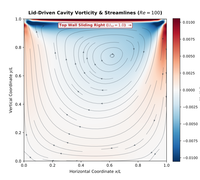
Building a Solver from Scratch

The core of CFD lies in its solver algorithms. Drawing on my coding background, I wanted to implement a minimal solver from scratch to observe firsthand how fluid states evolve at the discrete level and understand every microscopic state update. To verify that the implementation was free of fundamental errors, I tested it against a classic benchmark: the 2D lid-driven cavity flow—a square domain bounded by three stationary walls with a top lid moving horizontally at a constant velocity.

Starting with the Cavity Benchmark

For quantitative validation, I focused on steady-state $Re=100$ cavity flow across three grid resolutions: $32^2$, $48^2$, and $64^2$. I compared centerline velocity profiles against the benchmark data of Ghia, Ghia, and Shin (1982) while tracking convergence residuals and global mass conservation drift.

The web-based interactive demo integrates this LBMSolver on a $96 \times 64$ rectangular lattice at a default $Re=400$. Experience the FlowLab interactive demo here.

Implementation Details

I adopted the standard two-dimensional D2Q9 lattice model. Each lattice node stores 9 discrete particle velocity distributions corresponding to the rest state, four cardinal directions, and four diagonal directions. The lattice weights are $w_0 = 4/9$ for the rest state, $w_{1..4} = 1/9$ for the cardinal axes, and $w_{5..8} = 1/36$ for the diagonals.

During each timestep, macroscopic density is recovered by summing all 9 distributions, and macroscopic velocity is obtained via momentum weighted sum. The equilibrium distribution $f_i^{eq}$ is then constructed from density, velocity, lattice vectors, and directional weights. The collision step relaxes the local distributions toward equilibrium, controlled by the relaxation time $\tau$ (BGK model).

Following collision, distributions stream to adjacent target nodes (push streaming). If a target node is a stationary solid boundary, the distribution bounces back along its incoming direction (halfway bounce-back). For the moving top lid, momentum transfer from wall velocity must be accounted for during reflection. After swapping distribution buffers, macroscopic quantities are recomputed, and vorticity is calculated via $\omega = \partial v/\partial x - \partial u/\partial y$.

Reynolds number determines kinematic viscosity in lattice units, which in turn sets the relaxation time $\tau$:

$$\nu = \frac{U_{lid} L}{Re}$$ $$\tau = 0.5 + 3\nu$$

As $\tau$ approaches 0.5, this single-relaxation-time (SRT-BGK) scheme becomes susceptible to numerical instabilities. The solver explicitly rejects configurations with $\tau \leq 0.5005$. In steady-state runs, convergence is monitored every 250 steps by computing the RMS change across velocity components, normalized by $U_{lid}$.

Initially, I made the mistake of directly overwriting macroscopic velocities along the top boundary after streaming. While the rendered velocity field appeared plausible, the distribution functions bouncing back into the fluid carried no momentum update—meaning macroscopic display changed while microscopic state remained decoupled. I resolved this by applying proper Zou–He moving wall momentum injection directly inside the bounce-back routine.

During the initial $48^2$ verification run capped at 20,000 steps, centerline velocities closely matched the reference curves, but the residual sat at $4.80 \times 10^{-7}$—failing the strict $2 \times 10^{-7}$ convergence criterion. Rather than loosening the threshold, I increased the iteration budget until formal numerical convergence was reached. Visual agreement with external references does not guarantee internal state convergence.

Multi-Grid Validation Results

With extended iteration budgets, all three grid resolutions satisfied the identical convergence criterion. The reported velocity errors represent RMSE calculated against benchmark coordinates; mass drift measures relative total mass change throughout the simulation:

Fluid Grid	Iterations	Final Residual	$u/U_{lid}$ RMSE	$v/U_{lid}$ RMSE	Relative Mass Drift
$32^2$	14,750	$1.85\times10^{-7}$	0.00511	0.00404	$1.49\times10^{-12}$
$48^2$	22,000	$1.91\times10^{-7}$	0.00369	0.00208	$2.13\times10^{-12}$
$64^2$	27,500	$1.89\times10^{-7}$	0.00286	0.00202	$2.56\times10^{-12}$

Benchmark data sourced from Ghia, Ghia & Shin (1982), Journal of Computational Physics 48(3), 387–411 (DOI).

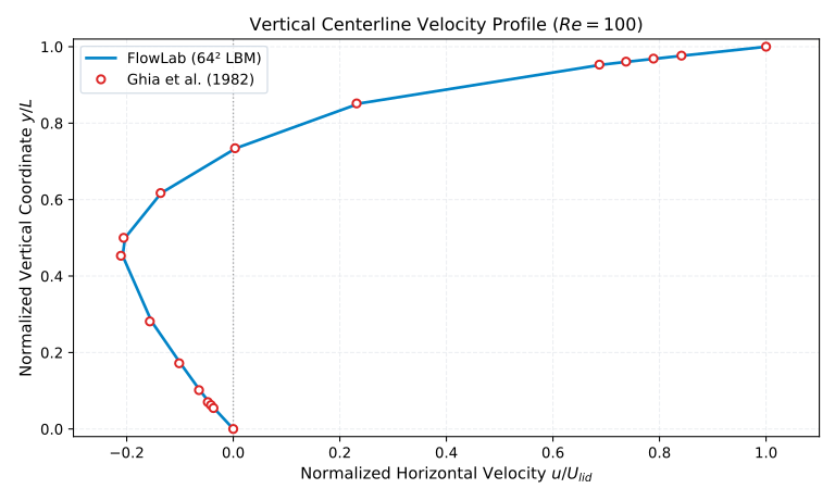
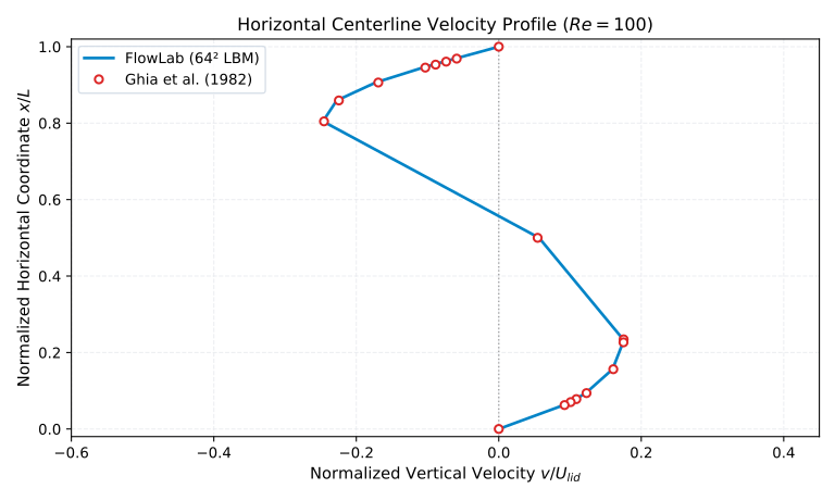
On the $64^2$ grid, RMSE along both centerlines remains below 1% of lid velocity, and total mass drift is contained below $10^{-9}$. Residuals verify internal steady-state convergence, Ghia benchmarks verify spatial velocity accuracy, and mass drift confirms global conservation. A plausible-looking vorticity contour cannot replace quantitative checks—an incorrect boundary implementation can still yield visually fluid-like vortices. Thus, vorticity plots serve only for qualitative structure inspection.

Web Interactive Demo

The web demo instantiates the lightweight LBMSolver on a $96 \times 64$ lattice. The interface allows selecting $Re = 100$, $400$, or $1000$, toggling between velocity and vorticity visualizations, pausing, resetting, and interacting with the flow via mouse or touch dragging.

The rendering loop invokes solver.step(1) per animation frame and renders directly from velocity or vorticity buffers. Interactive dragging calls setVelocityAt, modifying local macroscopic velocity and locally reconstructing the 9 equilibrium distributions. On an Apple M1 MacBook, the $64^2$ verification benchmark completed 27,500 steps in 4.21 seconds—translating to approximately 26.8 million node updates per second (MNUPS).

Downstream Application: FlowROM

When later developing FlowROM, I required a series of unsteady snapshot datasets to test model order reduction workflows. FlowLab’s ability to inject periodic boundary disturbances and export transient fields made it a practical data source for that work. However, this downstream application does not change the scope of FlowLab: it remains an educational project built to understand minimal solver architecture.

Several limitations remain: only the steady $Re=100$ cavity has undergone strict quantitative validation. The single-relaxation-time (SRT) BGK model becomes numerically fragile near $\tau = 0.5$; halfway bounce-back introduces grid-dependent effective wall placement; and lattice units have not yet been mapped to dimensional physical time.

Code and Reproduction

The codebase is open source on GitHub: gaoflow/flowlab

git clone https://github.com/gaoflow/flowlab.git
cd flowlab
npm test
npm run validate