How to Estimate Cooling Loop Flow Rate Without Physical Hardware

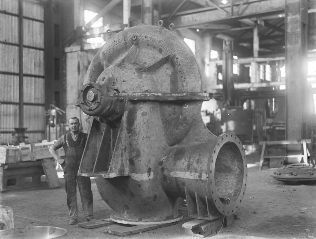
40 L/min on the Datasheet $\neq$ Real-World Flow Rate

This project was completed during my third month as a first-year M.S. student in Mechanical Engineering. The team was designing the cooling system for an FSAE race car. The water pump datasheet specified a “maximum flow rate of 40 L/min,” and I was tasked with evaluating what that 40 L/min actually translates to in practice.

This maximum flow rating assumes ideal conditions: essentially zero backpressure at the outlet. Once installed in the vehicle, the coolant must pass through hoses, elbows, a radiator, and narrow engine channels. It behaves much like a garden hose: when short and straight, it fills a bucket quickly; extend it, introduce bends, or pinch a section, and the flow rate drops significantly despite using the same water source.

If the flow rate is overestimated at this stage, any subsequent thermal calculations—no matter how many decimal places are retained—will be based on an incorrect operating condition. Thus, I set out to solve this core question:

Given a pump performance curve and a series cooling loop, at what flow rate does the pressure head delivered by the pump exactly balance the total system pressure loss?

The Fluid Circuit

To evaluate the flow rate, I discretized the loop into four sequential segments: the suction hose, the radiator core, the engine water jacket, and the return hose. They are connected in series, meaning fluid flows through each segment sequentially before returning to the pump.

A series circuit simplifies the analysis: the volumetric flow rate is identical across all segments. By calculating the pressure loss within each individual segment and summing them up, the total system head loss for a given flow rate can be obtained.

Component	Length ($L$)	Inner Diameter ($D$)	Minor Loss Coefficient ($K$)
Suction Hose	0.40 m	16 mm	1.5
Radiator Core	0.15 m	16 mm	8.0
Engine Water Jacket	0.50 m	14 mm	4.0
Return Hose	0.60 m	16 mm	2.0

The radiator introduces substantial flow resistance because coolant does not pass through a wide open cavity; instead, it is split into numerous narrow micro-channels.

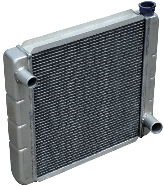
Converting Components to Pressure Drops

I applied the Darcy–Weisbach formulation to compute the pressure drop across each individual component:

$$\Delta p=\left(f\frac{L}{D}+K\right)\frac{\rho V^2}{2}.$$

This equation can be divided into two main components: $fL/D$ accounts for the major friction losses along the pipe walls, while $K$ accounts for minor losses introduced by bends, inlets, and internal geometry changes. The dynamic pressure term, $\rho V^2/2$, scales with flow velocity; higher velocities lead to quadratically higher pressure drops. While length, diameter, density, and velocity can be directly substituted, determining the Darcy friction factor ($f$) requires careful treatment. Rather than immediately solving the entire loop, I verified the calculation of $f$ independently first.

Friction Factor ($f$) Calculations

For laminar flow regime, $f$ is solved explicitly:

$$f=\frac{64}{Re}.$$

Here, the Reynolds number ($Re$) serves as a metric for the flow regime: at lower values, viscous forces dominate; at higher values, the flow transitions to turbulence, where pipe wall roughness begins to dictate friction losses. I sampled 200 points across $Re = 100$ to $2300$, and the solver’s numerical output matched $64/Re$ with zero residual error ($0.0$).

Turbulent flow is more complex. In the implicit Colebrook equation, $f$ appears on both sides of the equation, requiring iterative solution techniques. I used the Haaland approximation to generate an accurate initial guess, followed by Newton-Raphson iterations to refine the root. If convergence is not reached within 50 iterations, the program raises an exception rather than returning an invalid result. After solving, each evaluated $f$ was substituted back into the original Colebrook equation. Across 150 combinations of Reynolds numbers (up to $Re = 10^8$) and relative roughness values, the maximum residual was $3.55\times10^{-15}$, confirming the mathematical validity of the solver.

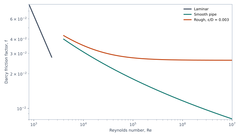
Domain Validation & Boundary Checks

As a secondary validation path, I implemented the explicit Swamee–Jain equation. While it claims an accuracy within $\pm3\%$, this guarantee is strictly bounded by the following domain:

$$5\times10^3\le Re\le10^8,\qquad 10^{-6}\le\varepsilon/D\le10^{-2}.$$

During initial testing, I evaluated points outside these specified boundaries. Near low relative roughness and $Re \approx 4\times10^3$, discrepancies between the Colebrook solver and Swamee–Jain exceeded 3%. Initially suspecting a bug in my Colebrook solver, further inspection revealed that these evaluation points fell outside the valid domain of the Swamee–Jain approximation. Once the validation test range was constrained strictly to the published validity domain, the maximum relative discrepancy dropped to 2.83%. This discrepancy did not require modifying the Colebrook solver, but rather adjusting the test envelope. It served as a good reminder: analytical reference formulas have operational boundaries and cannot serve as universal ground truth outside their specified domains.

With the friction factor solver fully validated across both tests, the four pipe segments could be integrated back into the complete circuit model.

Determining the Operating Point

Starting with an initial trial flow rate, I calculated the pressure drop across all four segments and summed them to obtain the total system resistance:

$$\Delta p_{sys}(Q)=\sum_i \Delta p_i(Q).$$

Repeating this calculation across a range of flow rates yields the system curve. Because flow resistance increases with velocity, the system curve slopes upward. Conversely, the pump supplies energy to the fluid, represented by a pump performance curve. In the physical vehicle, the pump impeller is driven by the engine crank via a belt and pulley. However, a pump cannot deliver a constant flow rate regardless of backpressure. In this model, a surrogate quadratic curve was used to approximate the pump characteristics:

$$\Delta p_{pump}=90\ \text{kPa}-cQ^2.$$

This curve yields a shut-off head of 90 kPa at zero flow and drops to zero head at 40 L/min (free delivery). The actual operating flow rate corresponds to the intersection of the pump curve and the system curve:

$$\Delta p_{pump}(Q)-\Delta p_{sys}(Q)=0.$$

The solver uses the Newton-Raphson method to locate this intersection point. If an iterative step projects outside the valid domain, the algorithm falls back to a bisection method to guarantee convergence.

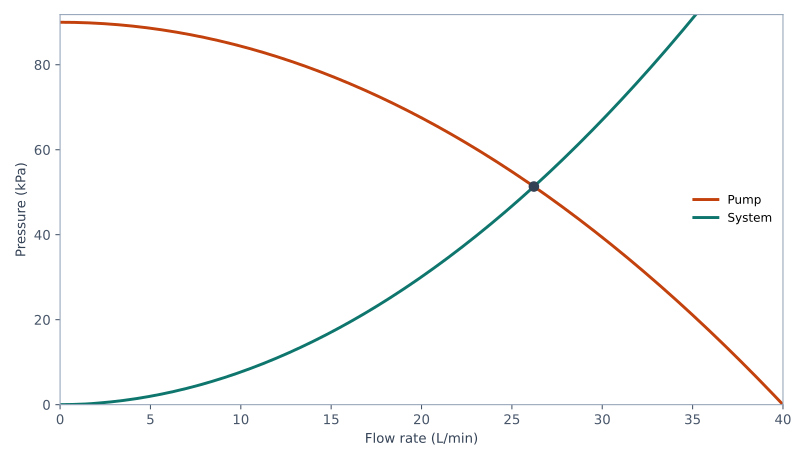
The two curves intersect at 26.22 L/min and 51.34 kPa. Under these simplified system parameters, connecting the 40 L/min free-delivery pump into the circuit results in an approximate 34% reduction in actual delivered flow.

High floating-point precision in numerical solvers does not automatically guarantee physical accuracy. To double-check the result, I performed a brute-force sweep over 4,096 uniformly spaced points between 0 and 40 L/min to locate the zero-crossing interval. This coarse scan bracketed the intersection between 26.2173 and 26.2271 L/min, closely matching the Newton-Raphson result. At this solved operating point, the residual difference between pump pressure and system head loss was less than $2.18\times10^{-11}$ Pa. Additional physical sanity checks were confirmed: system pressure drop monotonically increases with flow rate; introducing an additional 10 kPa of static head reduces the operating flow rate; and total loop pressure drop strictly equals the sum of the four individual segment losses. With the intersection point verified, the investigation turned to identifying the primary sources of pressure loss.

Pressure Loss Breakdown (51.34 kPa)

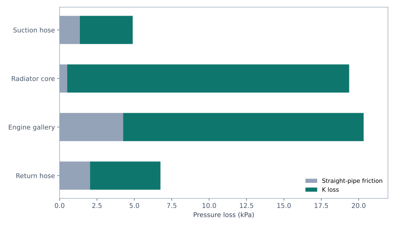
At the operating point, the pressure loss breakdown across components is as follows:

• Suction Hose: 4.89 kPa
• Radiator Core: 19.37 kPa
• Engine Water Jacket: 20.33 kPa
• Return Hose: 6.75 kPa

Combined, the radiator core and engine water jacket account for 39.70 kPa, or approximately 77% of the total loop pressure drop. Looking at loss mechanisms across the entire circuit, minor losses ($K$-factors) contribute 43.19 kPa (84.1%), whereas major friction losses ($fL/D$) account for only 8.14 kPa (15.9%).

Consequently, under this baseline configuration, reducing restriction in the radiator core and engine passages offers a significantly higher return on flow rate optimization than trimming hose lengths. Note that this insight holds specifically for the assumed geometry and loss coefficients; actual proportions may shift with empirical component data.

Key Takeaways

In summary, a rated value of 40 L/min represents only the free-delivery capacity of the pump under near-zero backpressure. When integrated into a real circuit, the actual operating point drops to 26.22 L/min at 51.34 kPa—a loss of over one-third of the rated flow. Furthermore, the loss breakdown revealed that ~77% of the total head loss originates within the radiator core and engine water passages, highlighting these areas as primary targets for flow optimization.

When evaluating a nominal flow specification, it is essential to determine the corresponding head loss and compare it against the system resistance curve. Flow rate is meaningful only when evaluated at the operating point where the pump curve intersects the system curve. Additionally, the Swamee–Jain discrepancy highlighted an important engineering lesson: when numerical results diverge, both the numerical solver implementation and the validity limits of empirical reference formulas must be audited.

Naturally, 26.22 L/min is not necessarily the final target flow rate for the actual vehicle. Several simplifications were made in this study: the pump curve was modeled as a surrogate quadratic equation, minor loss coefficients ($K$) were sourced from engineering handbooks rather than bench test measurements, and the fluid model assumed steady-state, incompressible, single-phase flow (omitting cavitation risk, air entrainment, NPSH checks, and parallel branching). Next steps involve incorporating empirical pump performance curves, measured component pressure drop data, parallel flow loops, and integrated thermal network models for further verification.

Code

The complete source code and test suite are available at gaoflow/pipe-flow-sizing:

git clone https://github.com/gaoflow/pipe-flow-sizing.git
cd pipe-flow-sizing
python3 -m unittest discover -s tests -v
python3 scripts/analyse.py

References: Governing formulas include the Haaland friction factor approximation, Swamee–Jain cross-validation explicit relation, and the original Colebrook paper.